
The Trip Distribution Analysis of Water Trucks as Heavy Vehicles
with PTV Visum Application
Zulfiani Ar, Anie Tuati and Amy Wadu
Politeknik Negeri Kupang, Kupang City, NTT, Indonesia
Keywords: Trip Distribution, Visum, DCGR Model.
Abstract: Water is the basic need of people and it supports the basic activities of the community in Kupang City.
Therefore, in order to meet the need for clean water, communities purchase water that is delivered by water
trucks and sold by private sectors. These heavy vehicles pass through public roads, increase the traffic volume
and affect the road capacity. This study aims to determine the trip distribution of heavy water trucks using the
Origin-Destination Matrix (ODM). The method used in analyzing the trip distribution is the Double
Constrained Gravity (DCGR) model with a negative exponential impedance function, which is then used to
assign the road network traffic in the PTV Visum Application. The resulting trip distribution model is Tid =
Oi.Dd.Ai.Bd.exp(-0,6181.Cid) and the total trip distribution of water trucks is at the rate of 131 vehicles/day.
The prediction of trip distribution shows that the highest traffic assignment is found on the Liliba village to
Oepura village route.
1 INTRODUCTION
Transportation difficulties, especially in developing
countries, continue to increase as the needs of
adequate transportation grow. Thus, in order to be
better prepared in fulfilling the need for transportation
infrastructure in the future, it is necessary to study the
trip patterns (Suthanaya and Maulidawati, 2019). The
acceleration of digital system also enhances the
opportunity to create a high-quality transportation
system (Maget et al., 2019).
A research conducted in Denpasar, Bali predicts
that the trip distribution will reach the total number of
28,873,490 people/day by 2033 (Suthanaya and
Maulidawati, 2019). In order to describe the trip
distribution of travelers in an area, it is necessary to
generate the Origin-Destination Matrix (ODM)
through conducting the Origin-Destination Survey.
Previous studies have also produced approximations
of trip distribution in West Java Province based on the
results of statistical tests using the Double
Constrained Gravity (DCGR) model with a negative
exponential impedance function, Tid =
Oi.Dd.Ai.Bd.exp
(-0,014159.Cid)
. (Aprilliansyah and
Herman, 2015).
This study aims to determine the trip distribution
of water trucks using the Origin-Destination Matrix
(ODM). The data is based on a survey of the water
trucks’ trip distributions starting from the water
sources, as the origin zones, to the points of delivery,
as the destination zones. Moroever, a research in the
City of El Paso, the United States, offers a model for
transportation planners to calculate the total trip
distribution (Bencomo, 2018). PTV Visum
application is an example of the utilization of
computerized traffic model and it provides modelling
of transport networks and transport demand,
including trip production-attraction and spatial trip
distribution (Jacyna, 2017).
2 LITERATURE REVIEW
2.1 Origin-Destination Matrix
In the transportation system, trip patterns are often
described in terms of the trip flow of vehicles,
passengers, and goods that move from the origin zone
to the destination zone within a certain area and over
a certain period of time. The Origin-Destination
Matrix is often utilized by transport planners to
describe these trip patterns.
Origin-Destination Matrix is a two-dimensional
matrix that contains information of trips between
1056
Ar, Z., Tuati, A. and Wadu, A.
The Trip Distribution Analysis of Water Trucks as Heavy Vehicles with PTV Visum Application.
DOI: 10.5220/0012057300003575
In Proceedings of the 5th International Conference on Applied Science and Technology on Engineering Science (iCAST-ES 2022), pages 1056-1061
ISBN: 978-989-758-619-4; ISSN: 2975-8246
Copyright © 2023 by SCITEPRESS – Science and Technology Publications, Lda. Under CC license (CC BY-NC-ND 4.0)
zones in a certain area. The row denotes the origin
zone, the column represents the destination zone, thus
the cells represent the amount of trip from the origin
zone to the destination zone. In this case, the notation
states the amount of trip flow (vehicles,
passengers, or goods) from the origin zone i to the
destination zone d during a certain time interval. Trip
patterns can be generated if the Origin-Destination
Matrix is utilized in a transport network system. By
examining the trip patterns, the transport problems
can be identified and solutions may be immediately
generated.
The Origin-Destination Matrix plays a pivotal
role in transport planning and management as it
provides a detailed explanation of the trips. The
number of zones and the value of each cell are two
most important elements in Origin-Destination
Matrix, as the number of zones indicates the total
number of cells that can be obtained. Each cell
requires information on distance, time, cost, or a
combination of these three, which is used as a
measure of accessibility. The general form of the
Origin-Destination Matrix can be seen in Table 1.
2.2 Trip Distribution
Trip distribution is the flow of trip production from
one zone to a number of other zones, known as zone-
to-zone trip. Several methods can be used to generate
the trip distribution, including the Synthetic Method.
The widely known, and frequently used, synthetic
method (spatial interaction) is the gravity model (GR)
as it is rather simple and easy to understand. This
model follows the concept of gravity introduced by
Newton in 1686. This method assumes that the
production and attraction of trips are related to several
parameters of the origin zone, such as population and
accessibility, including distance, time, or cost. The
accessibility is regarded as an impedance and is
calculated using a negative exponential function.
Table 1: The general form of Origin-Destination Matrix.
Zona 1 2 3 … N O
i
1 T
11
T
12
T
13
… T
1N
O
1
2 T
21
T
22
T
23
… T
2N
O
2
3 T
31
T
32
T
33
… T
3N
O
3
. . . . … . .
. . . . … . .
. . . . … . .
N T
N1
T
N2
T
N3
… T
NN
O
N
D
d
D
1
D
2
D
3
… D
N
T
The β parameter is obtained from the quotient
between the value of K which ranges from 2~3 with
, which is the average of the impedance value
(Aprilliansyah and Herman, 2015).
()
=
()
(1)
Double-constrained Gravity Model (DCGR) is
used in the equation (1) (Tamin, 2000).
=
.
.
.
.
()
(2)
Dimana:
= number of trips between zone i and d
(trips/day)
= number of trips from origin zone i
(trips/day)
= number of trips from destination zone d
(trips/day)
= production balancing constant
= attraction balancing constant
()
= impedance function
With the boundary conditions can be seen in
equation (3) and equation (4).
=
1
∑
(
.
.
()
)
(3)
=
1
∑
(
.
.
()
)
(4)
2.3 PTV Visum
PTV Visum is a world's leading software for
macroscopic modelling of transportation and is
currently used by more than 1,000 organizations. It
provides transportation modelling of the traffic
network, as well as a feature to analyze the external
effects of traffic, such as air pollution and noise levels
(AR, 2021).
The traffic assignment can be modelled in the
PTV Visum application and the result can be used as
the measurement for the road segment and the road
network. This stage involves three components,
namely the trip matrix, the road network, and the
assignment mechanism, including the route selection
and the road restriction for goods transport vehicles
(Citra et al., 2019).
Trip distribution is part of four sequential
transportation modelling steps. Trip production and
attraction are calculated by determining the
impedance matrix from the total requested trip. The
elements of the matrix itself are calculated under the
The Trip Distribution Analysis of Water Trucks as Heavy Vehicles with PTV Visum Application
1057
trip distribution procedure. On the one hand, the trip
distribution from the destination zone to the origin
zone is based on the attraction of the trip, on the other
hand the trip distribution from the origin zone to the
destination zone is measured by the matrix of travel
time, fares and other general costs (Visum 15, 2015).
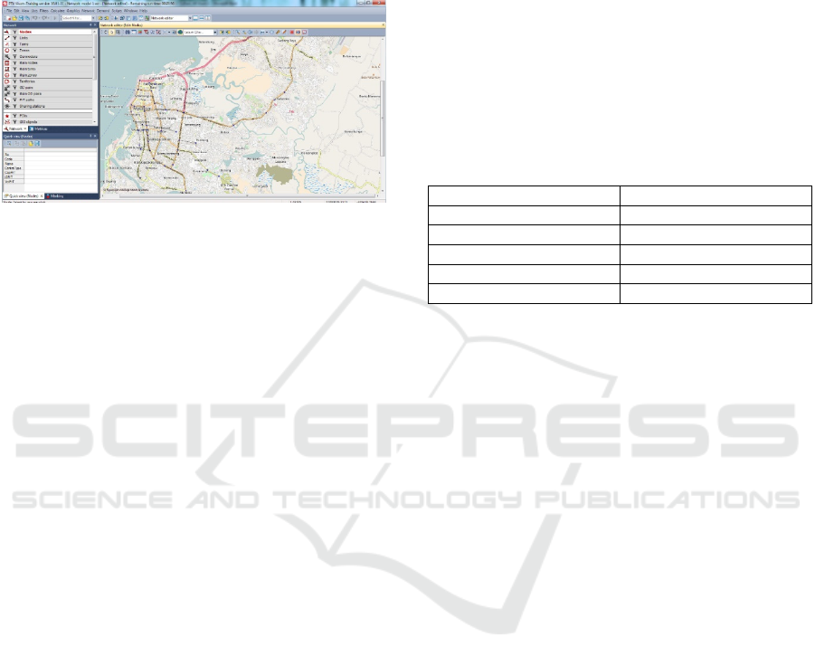
Figure 1: Example of an observation points map in the
VISUM Program (AR, 2021).
3 RESEARCH METHOD
This study begins with a preliminary research on the
volume of heavy vehicles, specifically of water trucks
in Kupang City. After conducting the preliminary
survey, it is necessary to identify how the volume of
the water trucks affects the road capacity. Thus, a
reference matrix is developed based on the topic and
research objectives. Following this, the data
collection process is conducted through direct
surveys, such as observations and interviews, as well
as filling a survey form at the origin zone and the
destination zone. The survey is conducted within five
working days, as the research location consists of five
zones, namely zone 1 (Oebobo), zone 2 (Kayu Putih),
zone 3 (Liliba), zone 4 (Oepura), and zone 5
(Oesapa).
The data summary and data processing steps are
completed through the Origin-Destination Matrix
with the help of Microsoft Excel. Furthermore, the
DCGR Model is used to calculate the trip distribution
and then the results are assigned into the road network
by the PTV Visum application. Once the trip
distribution data is obtained, the future policy on
traffic management may be formulated based on this
finding.
3.1 Trip Distribution Survey
The trip distribution survey is delivered by collecting
five types of data, namely the total number of heavy
vehicles, travel time, travel distance, and travel cost.
3.1.1 Heavy Vehicles Survey
This survey is conducted in five research zones, from
07 AM to 06 PM for five days, namely Oebobo
village, Sikumana village, Liliba village, Oepura
village, and Oesapa village which can be seen in
Table 2. The survey is carried out by identifying
water trucks in each origin zone (water collection
points) and the destination zone (end-consumer
delivery points). This study ensures each truck is
available to participate in the survey, recorded based
on the vehicle number, and shadowed by the surveyor
to the destination zone.
Table 2: Trip distribution zone.
Zone Village
1 Oebobo
2 Sikumana
3 Liliba
4 Oepura
5 Oesapa
3.1.2 Travel Time Survey
Travel time records the time needed for the water
trucks to arrive at the destination zone from the origin
zone. The travel time survey utilizes a basic,
smartphone-based timer application and the data is
taken from each zone and for each water truck.
3.1.3 Distance Survey
This survey records the distance from the origin zone
to the destination zone. The distance survey utilizes a
basic, smartphone-based distance tracker application
and the data is taken from each zone and for each
water truck.
3.1.4 Travel Cost Survey
This survey directly interviews water truck drivers on
the transportation cost needed to travel from the
origin zone to the destination zone. The data is taken
in each zone and for each water truck.
4 RESULTS AND DISCUSSION
The result of Origin-Destination Matrix (ODM) as the
output of the survey can be seen in Table 3. Based on
the matrix, the origin zone with the highest traffic is
zone 3 (Liliba village), which it records the rate of 38
vehicles/day. Meanwhile, zone 1 (Oebobo village) is
the origin zone with the second highest record of trips
iCAST-ES 2022 - International Conference on Applied Science and Technology on Engineering Science
1058
at 29 vehicles/day. Furthermore, Zone 5 (Oesapa
village) is the third highest origin zone with a trip rate
of 25 vehicles/day.
On the other hand, Zone 5 (Oesapa village) is the
destination zone with a highest trip record of 34
vehicles/day. The second position is held by zone 3
(Liliba village) with the value of 29 vehicles/day.
Moreover, zone 4 (Oepura village) is the third busiest
destination zone with a record of 24 vehicles/day.
The origin zone with the least trip distribution is
zone 4 (Oepura village), with a record of 18
vehicles/day. While the destination zones with the
least trip distributions are zone 1 (Oebobo village)
and zone 2 (Sikumana village), both record the value
of 22 vehicles/day.
Meanwhile, the number of trips from the origin
zone to the destination zone with the highest number
of trips (Oesapa village) is 23 vehicles/day. The rate
of 1 vehicle/day from the origin zone to the
destination zone with the least trip distribution, is
shown by Oebobo to Sikumana and Liliba village;
Sikumana to Oebobo, Liliba, Oepura and Oesapa
village; Liliba to Sikumana and Oepura; Oepura to
Liliba village; and Oesapa to Oebobo and Sikumana
village.
Table 3: The result of Origin-Destination Matrix (ODM) of
water trucks.
Zone 1 2 3 4 5 O
i
1 6 1 1 15 6 29
2 1 17 1 1 1 21
3 3 1 23 1 10 38
4 11 2 1 2 2 18
5 1 1 3 5 15 25
D
d
22 22 29 24 34 131
The table shows that Liliba village has a high trip
distribution, as the result of abundant water resources
in this particular zone and adequate road accessibility.
Meanwhile, Oesapa village shows that the community
has a high demand for clean water, although the
demand originates internally or from the same zone.
4.1 Impedance Function Analysis
Distance, as one of the accessibility functions, is
regarded as an impedance function that will illustrate
the longest and shortest distance taken by the water
trucks. As seen from the table 4, the shortest distance
is recorded between zone 2 (Sikumana village) to zone
1 (Oebobo village) because the road access is adequate
enough. On the contrary, the longest distance is
recorded between the zone 2 (Sikumana village) to
zone 5 (Oesapa village) as both points are far apart.
Table 4: Accessibility matrix (
).
Zone 1 2 3 4 5
1
1,93 5,40 3,40 0,88 2,13
2
0,45 1,53 5,45 0,88 12,60
3
3,43 2,90 1,54 5,50 0,96
4
2,86 2,55 4,10 0,98 5,60
5
5,40 3,00 2,83 2,34 2,26
Table 5 displays the value of the impedance
function for each zone of origin and destination using
a negative exponential function with a value of
of
3.236 and β with the value of 0.6181.
Table 5: Accessibility function matrix (
()
).
Zone 1 2 3 4 5
1 0,3027
0,0355 0,1223 0,5817 0,2675
2
0,7572 0,3880 0,0344 0,5823 0,0004
3
0,1198 0,1666 0,3862 0,0334 0,5542
4
0,1706 0,2068 0,0793 0,5474 0,0314
5
0,0355 0,1566 0,1736 0,2354 0,2474
4.2 DCGR Model Analysis
The Origin-Destination Matrix (ODM) is then
analysed with the DCGR model by entering the
calculated distance as the impedance function. The
data is processed using the value of
and
alternately for each origin and destination zone.
The iteration process starts by assuming the values of
,
,
,
, dan
= 1. The iteration is repeated
14 times until the values of each
and
reach
convergence, or static, including in the next iteration.
The results then act as the input for the Origin-
Destination matrix using Equation (2). Hence, the
water trucks’ trip distribution in the form of DCGR
model can be seen in Table 6.
The Origin-Destination Matrix, generated from
the DCGR model, illustrates the trip distribution of
water trucks with a distance factor. The results show
that there is a difference between the ODM based on
the preliminary calculation and the ODM based on
the DCGR model. A significant change is seen in
zone 1 (Oebobo village) with a decrease from 15
vehicles/day to 8 vehicles/day due to the long
distance between Oebobo village and Oepura village.
Additionally, zone 2 (Sikumana village) also
experiences a change with a decrease from 17
vehicles/day to 6 vehicles/day. This is because the trip
distribution is more evenly generated based on the
distance.
The Trip Distribution Analysis of Water Trucks as Heavy Vehicles with PTV Visum Application
1059
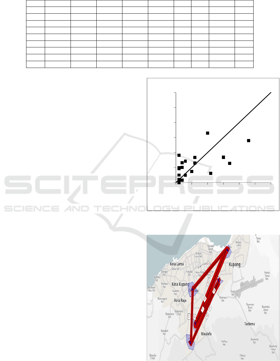
Table 6: Origin-Destination Matrix of water trucks generated from DCGR model.
Zone 1 2 3 4 5 o
i
O
i
A
i
E
i
1 7 1 5 8 8 29 29 0,0330 1,00
2 9 6 1 5 0 21 21 0,0256 1,00
3 2 5 14 0 16 38 38 0,0240 1,00
4 3 5 3 7 1 18 18 0,0442 1,00
5 1 5 7 4 8 25 25 0,0415 1,00
d
d
22 22 29 24 34
131
D
d
22 22 29 24 34
131
B
d
1,0226 1,3871 1,3686 0,6334 0,9589
E
d
1,00 1,00 1,00 1,00 1,00
1,00
Furthermore, zone 3 (Liliba village) also
experiences a change of trip distribution due to the
distance factor between zones, from 10 vehicles/day
to 16 vehicles/day.
The largest change occurs in the destination zone
1 (Oebobo village) with a decreasing value from 11
vehicles/day to 3 vehicles/day due to a long distance
between these two zones. Also, the most significant
trip distribution value change in zone 5 (Oesapa
village) occurs inside the destination zone 5 itself
where the value of 15 vehicles/day decreases to 8
vehicles/day. This is because the trip distribution is
more evenly generated based on the distance.
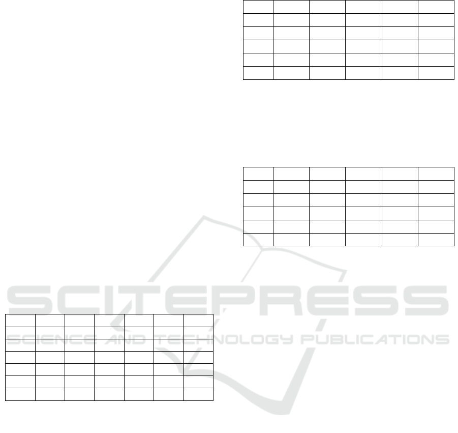
The comparison of the Origin-Destination Matrix
based on the preliminary calculation and the one
generated by the DCGR model can be seen in Figure
2. The results of the comparison then create the
equation Y = 3.074 + 0.413X with a correlation
coefficient value (r) = 0.629. This illustrates that the
Origin-Destination Matrix based on the preliminary
calculation and the origin-destination matrix based on
the DCGR model has a fairly close correlation.
4.3 Assigning with PTV Visum
The origin-destination matrix based on the DCGR
model is utilized to assign the trip distribution to the
road network using the PTV Visum application. The
data needed in the application is the zone data for each
village which is stored as node, link, zone, and
connector, as well as the Origin-Destination Matrix
of the DCGR model. The traffic characteristics such
as the initial capacity and initial speed is obtained
from secondary data. Meanwhile, data on travel time
is obtained from surveys.
The assignment of the Origin-Destination Matrix
is calculated using the Equilibrium Assignment
method. The map of water trucks’ trip distribution,
with a line of demand connecting the origin zone and
the destination zone, can be seen in Figure 3.
Figure 2: Comparison of ODM with preliminary calculation
and ODM with DCGR model.
Figure 3: The results of assigning trip distribution with the
PTV Visum Application.
0
5
10
15
20
25
30
0 5 10 15 20 25 30
T
id
DCGR Model (vehicle/day)
T
id
Calculation (vehicle/day)
0
5
10
15
20
25
30
0 5 10 15 20 25 30
T
id
Model DCGR (kend/hari)
T
id
Pengukuran (kend/hari)
iCAST-ES 2022 - International Conference on Applied Science and Technology on Engineering Science
1060

In addition to the map of trip distribution, the PTV
Visum application also generates the data of vehicles
volume at each link that connects origin zone and
destination zone. Based on Table 7, the largest
volume is shown on the trip from origin zone 3 to the
destination zone 4, which is from Liliba village to
Oepura village, at the rate of 21 vehicles/day.
Meanwhile, the smallest volume is located on the trip
from origin zone 1 (Oebobo village) to destination
zone 2 (Sikumana village), origin zone 2 (Sikumana
village) to destination zone 1 (Oebobo village), origin
zone 2 (Sikumana village) to destination zone 3
(Liliba village), at the rate of 11 vehicles/day.
Table 7: Vehicles volume for each origin zone and
destination zone generated by the PTV Visum Application.
Origin
Zone
Destination
Zone
Volume
(vehicle/day)
1 2 11
2 1 11
2 3 11
3 2 12
3 4 21
4 3 15
4 5 20
5 4 19
1 5 16
5 1 9
5 CONCLUSIONS
The total trip distribution of water trucks from all
zones combined is at the rate of 131 vehicles/day.
Furthermore, the origin-destination matrix
calculation based on the DCGR model generate a trip
distribution model Tid = Oi.Dd.Ai.Bd.exp
(-0,6181.Cid)
.
The prediction of trip distribution shows that the
highest traffic assignment is found on the Liliba
village to Oepura village route, at the rate of 21
vehicles/day. Furthermore, alternative options, in the
form of modeling and traffic engineering, are crucial
in order to anticipate the increasing number of heavy
vehicles, such as water trucks, on certain routes.
ACKNOWLEDGEMENTS
DIPA Kupang State Polytechnic.
REFERENCES
A. Citra, J. Pangaribuan, U. W. (2019). Penentuan Lintas
Angkutan Barang di Kota Kupang.
Aprilliansyah, T., & Herman. (2015). Perkiraan Distribusi
Pergerakan Penumpang di Provinsi Jawa Barat
Berdasarkan Asal Tujuan Transportasi Nasional. Jurnal
Online Institut Teknologi Nasional, 1(1), 29–40.
AR, Z. (2021). Prediksi Kebisingan Lalu Lintas Heterogen
Menggunakan Aplikasi Visum. Macca Umi, 6(2).
Jacyna, M., Wasiak, M., Kłodawski, M., & Gołȩbiowski, P.
(2017). Modelling of Bicycle Traffic in the Cities Using
VISUM. Procedia Engineering, 187, 435–441.
https://doi.org/10.1016/j.proeng.2017.04.397
Maget, C., Pillat, J., & Waßmuth, V. (2019). Transport
demand model for the Free State of Bavaria-basis for
local transport planning. Transportation Research
Procedia, 41(2016), 219–228. https://doi.org/10.1016/
j.trpro.2019.09.040
Suthanaya P, A., & Maulidia, C. (2019). Analysis of travel
pattern in denpasar city. A Scientific Journal Of Civil
Engineering, 23(1411–1292), 1–8.
Tamin, O. z. (n.d.). Perencanaan & Pemodelan
Transportasi.
Manual PTV Visum 15.2015. PTV AG: Jerman.
Vidana-Bencomo, J. O., Balal, E., Anderson, J. C., &
Hernandez, S. (2018). Modeling route choice criteria
from home to major streets: A discrete choice approach.
International Journal of Transportation Science and
Technology, 7(1), 74–88. https://doi.org/10.1016/j.ijtst.
2017.12.002
The Trip Distribution Analysis of Water Trucks as Heavy Vehicles with PTV Visum Application
1061
