
Analysis of the Seismic Destructive Force and Building Features with
Tree-Based Machine Learning
Yingquan Lei
University College London, London, England, WC1H 9BT, U.K.
Keywords: Earthquake, Building Features, Data Analysis, Machine Learning.
Abstract: Earthquakes have long been highly destructive and can cause huge economic losses and casualties. It is natural
that people hope to predict earthquakes in advance so as to avoid losses. Whereas earthquake is a very complex
geographical phenomenon to predict and the data required is not sufficient currently, so, unfortunately, there
is no accurate prediction method yet. However, there is something worth exploring from the perspective of
building characteristics, which is more controllable and easier to study compared to the mysterious
earthquake. And so far, little research has been conducted about the connection between building features and
earthquake damage. In this paper, first, with the help of some python visualization tools, several representative
building features are analyzed, giving possible solutions to targeted disaster relief as well as how to improve
the seismic ability. The first few most important features are found and the significance is quantified. Then
machine learning is involved to predict the damage, and the optimal algorithm has a 72% accuracy rate.
1 INTRODUCTION
In April 2015, a 7.8 magnitude earthquake occurred
near the Gorkha district of Gandaki Pradesh, Nepal.
Almost 9000 lives were lost, millions of people were
instantly made homeless, and $10 billion in damages-
roughly half of Nepal’s nominal GDP-were incurred.
Since then, the Nepalese government has worked
intensely to help rebuild the affected district’s
infrastructures. Throughout the process, the National
Planning Commission, along with Kathmandu living
labs and the Central Bureau of Statistics, has
generated one of the largest post-disaster datasets
ever collected, containing valuable information on
earthquake impacts, household conditions, and socio-
economic-demographic statistics.
Two versions of the data, V1 and V2, are gathered
for different purposes. The goal is to study the
relations between the properties of buildings and the
earthquake damage grade, for which there are 2 sub-
tasks to be done. First, exploratory data analysis
(EDA) is carried out to give a deeper understanding
of the datasets, generate some results, and provide
valuable insights for the following machine learning
task. Then, information about buildings before the
earthquake is used to predict the damage it caused. In
the EDA part, some useful information will be
extracted with the help of figures plotted by python.
Based on the extracted information, possible causes
are discussed, the correlation between variables is
analyzed, the most important features are found, and
the significance is discussed by a comparative
analysis. In the machine learning part, the input is
optimized and hyperparameters are tuned to reach a
better accuracy rate. The study is conducted both for
the residence and the government, in the hope that
building features and the seismic ability of the
residence can be better adjusted and improved, and
the guideline for targeted disaster relief after the
earthquake can be better set by the government to
save lives in time and reduce the potential loss.
2 EDA ON DATASETS
This part is basically done by python visualization
tools (matplotlib, plotly, seaborn) on the split training
set. The purpose of the splitting is to avoid data
snooping. Data snooping occurs when a given set of
data is used more than once for purposes of inference
or model selection. When such data reuse occurs,
there is always a possibility that any satisfactory
results obtained may simply be due to chance rather
134
Lei, Y.
Analysis of the Seismic Destructive Force and Building Features with Tree-Based Machine Learning.
DOI: 10.5220/0012071100003624
In Proceedings of the 2nd International Conference on Public Management and Big Data Analysis (PMBDA 2022), pages 134-141
ISBN: 978-989-758-658-3
Copyright
c
2023 by SCITEPRESS – Science and Technology Publications, Lda. Under CC license (CC BY-NC-ND 4.0)

than to any merit inherent in the method yielding the
results (White 2000).
2.1 Overview
As can be seen from Figure 1 and Figure 2, the
damage grade is divided into 3 and 5 levels in V1 and
V2 respectively. In either version the earthquake is
highly destructive: only 9.57% of the buildings are at
a low damage grade in V1 and only 21.7% are at the
grade 1 or grade 2 in V2.
Figure 1: Damage Grade Distribution in V1. Figure 2: Damage Grade Distribution in V2.
Table 1: V1 head (Shape of V1: 260601, 39).
building
_id
geo_level_
1_id
geo_level_
2_id
geo_level_3
_id
… has_secondary_
use_police
has_secondary_u
se other
damage_
grade
802906 6 487 12198 … 0 0 3
28830 8 900 2812 … 0 0 2
94947 21 363 8973 … 0 0 3
590882 22 418 10694 … 0 0 2
201944 11 131 1488 … 0 0 3
Table 2: V2 head (Shape of V2: 762093, 44).
building_id district_
id
vdcmun_i
d
ward_id … has_superstructure_rc
_engineered
has_Superstruct
ure_other
damage_g
rade
120101000011 12 1207 120703 … 0 0 3
120101000021 12 1207 120703 … 0 0 5
120101000031 12 1207 120703 … 0 0 2
120101000041 12 1207 120703 … 0 0 2
120101000051 12 1207 120703 … 0 0 1
2.2 Feature Analysis
In this part, relations between damage grades and
some representative building features are visualized
and discussed.
Age and Damage. As shown in Figure 3, the age
of the building correlates positively with the damage
grade as expected, and buildings are more vulnerable
to earthquake impact as age increases. Undoubtedly,
when doing targeted disaster relief, age is always a
valid feature to account for the damage. However,
age makes little difference after a certain value. In
this case, for example, after 15 years or so, age is no
longer a significant indicator of the damage grade.
Thus, the oldest buildings should not simply be given
top priority before considering other possible factors.
Analysis of the Seismic Destructive Force and Building Features with Tree-Based Machine Learning
135

Figure 3: The damage grade distribution for each age group.
A possible explanation is that some other factors
compensate for the age. Some old buildings are
forcibly demolished due to security considerations,
while others are refurbished, or they are carefully
designed during construction in order to last for a
long period. An example would be historical
buildings. They cost a lot of resources when
constructed, and normally, huge efforts are made by
the government in preservation due to their great
significance.
Area and Damage. According to Figure 4, the
area of the building and the damage grade are
generally negatively correlated, suggesting that,
during targeted disaster relief after the earthquake,
smaller buildings should be given a higher priority
compared with larger ones which are less likely to be
highly destructed.
Figure 4: The damage grade distribution for each area group.
A possible interpretation could be that buildings
large enough are more likely to be public buildings
such as hospitals, schools, airports, government
offices, or possibly a residence of the wealthy. Thus,
these buildings are more carefully designed in the
structure during construction. They tend to be built
with more durable materials and given better
maintenance. Even the land quality may be carefully
assessed in advance. The terms “large enough” and
“generally” are used here since, as above, the
tendency can hardly be recognized at first. For
instance, the change from “37%” to “36.2” is slight,
and even “8.51%” to “7.23%” contradicts the general
tendency. The data might be partly explained by the
fact that there are few public buildings in these area
groups. But the conclusion becomes much clearer as
the area gets larger.
Position and Damage. As Figure 5 shows, there
can be attachments to, at most, 3 sides of the building,
or there can be no attachments at all. The association
between the position and the damage grade of
buildings is less obvious when there are no
attachments or there are attachments to only one side
of the building. But a rough tendency can be seen that
the number of the attached side of the building
associates negatively with the damage grade.
Figure 5: Distribution of the damage grade by position.
PMBDA 2022 - International Conference on Public Management and Big Data Analysis
136
The data may be explained, to some extent, as a
result of the concurrent effect of the multi-factors
discussed above. With more sides being attached, the
buildings are more likely to be public buildings or
owned by the developers of large real estate, which
means the building itself has better features. Or on the
other hand, the attachment itself can enhance a
building’s seismic ability. This is a problem worth
exploring in the aspect of engineering.
2.3 The Search for Correlations
Correlation heat maps are plotted after encoding non-
numerical variables.
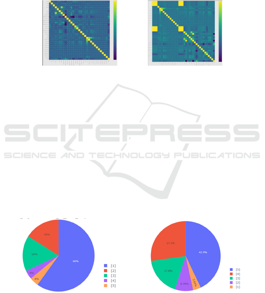
Figure 6: The correlation heat map of V1. Figure 7: The correlation heat map of V2.
As seen in Figure 6 and Figure 7, the height and
count on floors are positively correlated as expected,
with a correlation of 0.77. The use of superstructural
mud mortar stones and cement mortar bricks are
negatively related, with a correlation of -0.52. It is
worth noting that these two materials can not be
chosen at the same time since they are generally
different in firmness and not in the same price range.
Regarding the damage grade and features, the
post-eq features in V2 that are not of interest are
neglected, and the correlations of age and area are
0.027 and -0.12 respectively, which reconfirms the
conclusion drawn in the position and damage. Also,
the first few features with the strongest correlations
in the two versions are accordant as expected. They
are:
“has_superstructure_mud_mortar_stone”
”has_superstructure_cement_mortar_brick”
“has_superstructure_rc_engineered“
“has_superstructure_rc_non_engineered”
The correlation in V1 (0.29, -0.25, -0.18, -0.16) is
not as strong as that in V2 (0.48, -0.35, -0.21, -0.21).
There are some possible reasons. First, there are only
3 damage levels in V1 compared with 5 in V2, which
means changes in damage grades that can be
recognized in V2 are possibly still within the same
grade in V1. Also, the data volume of V1 is only one-
third of that of V2, probably leading to some bias.
Now the significance of the features listed above
will be discussed, where the significance represents
how big the difference in the damage grade
distribution is when optimal values are applied to the
building features. When the buildings have
superstructure _ cement _ mortar _ brick, rc _ non _
engineered, and rc _ engineered, and do not have
superstructure _ mud _ mortar _ stone, the
corresponding damage grade distribution is shown in
Figure 8. When the values are opposite, the
corresponding damage grade distribution is shown in
Figure 9.
Figure 8: The damage grade distribution with optimal
features.
Figure 9:The damage grade distribution with opposite
values.
Analysis of the Seismic Destructive Force and Building Features with Tree-Based Machine Learning
137

The improvement is quite significant: if grades 4
and 5 are considered as high damage grades and
grades 1 and 2 as low damage grades, the probability
of buildings getting a high damage grade is only 8%
after controlling these 4 features, compared with
70.2% taking opposite values, or 60.3% when the
building is randomly chosen in the area, according to
the overall damage distribution in Figure 2. Before
going into the conclusion, some definitions in which
the features involved should be made clear:
RC (Reinforced Concrete): most structures are
built by timber, steel, and reinforced (including
prestressed) concrete. Lightweight materials such as
aluminum and plastics are also becoming more
common in use. Reinforced concrete is unique
because the two materials, reinforcing steel and
concrete, are used together; thus the principles
governing the structural design in reinforced concrete
differ in many ways from those involving design in
one material (Wang, Salmon 1979).
Non-Engineered: non-engineered buildings are
defined as those that are spontaneously and
informally constructed in various countries in a
traditional manner with little intervention by
qualified architects and engineers (Arya 1994).
Therefore, a conclusion can be drawn that, to
improve the seismic ability in the area, the local
government should give top priority to improving the
quality of the construction material, specifically,
getting rid of the mud mortar stone and using the
cement mortar brick, reinforced concrete, or other
stronger materials instead. Also, interestingly,
buildings should better be both engineered, as
expected, and non-engineered in some other parts,
meaning that traditional methods, which may
incorporate some regional characteristics, should also
be taken into account during the construction. Once
these have been done, under a similar situation, the
risk of getting highly destructed (grade 4 and 5) will
plummet to around 1/8 of that of buildings with
features not intentionally controlled.
3 MACHINE LEARNING:
PREDICTING BUILDING
DAMAGES FROM FEATURES
By now, some conclusions have been drawn based on
the data analysis, which generates some insights that
are helpful in this part. Experiments and comparisons
will be carried out on both datasets.
3.1 Choosing Appropriate
Classification Algorithms
Four basic mainstream classification algorithms are
considered here: Support Vector Machines (SVM),
Naïve Bayes Classifier, Decision Tree Classifier
(DT), and Random Forest Classifier (RF).
Support Vector Machines (SVM). Applying
SVM requires input features expressible in the
coordinate system. In pattern recognition, the training
data are given in the form below:
(
x
,y
)
,…,
(
x
,y
)
∈R
×
+1, −1
(1)
These are n-dimensional patterns (vectors) x
and their labels y
. A label with the value of +1
denotes that the vector is classified to class +1 and a
label of -1 denotes that the vector is a part of class -1
(Busuttil 2003).
But both V1 and V2 contain many categorical
variables such as “ground_floor_type” and
“roof_type” which do not make sense in R
and
should not be simply discarded. Thus, SVM fails
here.
The Naïve Bayes Classifier. The nature of Naïve
Bayes assumes independence and involves the
calculating product of all features:
PXy
Py
=PX,y
=P(x
,x
,…,x
,y
)=
Px
x
,x
,…,x
,y
Px
,x
,…,x
,y
(2)
Because
P
(
a, b
)
=P
(
a
|
b
)
P
(
b
)
=
Px
x
,x
,…,x
,y
Px
|x
,x
,…,x
,y
Px
,x
,…,x
,y
=
Px
x
,x
,…,x
,y
Px
|x
,x
,…,x
,y
··· P(x
|y
)P(y
) (3)
Assuming that the individual x
is independent
from each other, then this is a strong assumption,
which is clearly violated in most practical
applications and is, therefore, naïve—hence the
name. This assumption implies that
Px
x
,x
,…,x
,y
=Px
y
, for example.
Thus, the joint probability of x and y
is (Berrar
2018):
PXy
Py
=Px
y
·Px
y
···
Px
y
Py
=
∏
Px
y
Py
(4)
However, correlation maps for both V1 and V2 in
Figure 6 and Figure 7 show several strong
correlations between variables. Also, since there are
many features, it might lead to a relatively large bias
during the calculation of the product. Naïve Bayes
will not be used here.
The Decision Tree Classifier (DT) and
Random Forest Classifier (RF). Instead, the
training will be conducted by tree-based algorithms,
say RF and DT, with the definition below:
Random forests are a combination of tree
predictors such that each tree depends on the values
PMBDA 2022 - International Conference on Public Management and Big Data Analysis
138

of a random vector sampled independently and with
the same distribution for all trees in the forest
(Breiman 2001).
This method classifies a population into branch-
like segments that construct an inverted tree with a
root node, internal nodes, and leaf nodes. The
algorithm is non-parametric and can efficiently deal
with large, complicated datasets without imposing a
complicated parametric structure. When the sample
size is large enough, study data can be divided into
training and validation datasets. Using the training
dataset to build a decision tree model and a validation
dataset to decide on the appropriate tree size needed
to achieve the optimal final model (Song, Lu 2015).
3.2 Feature Engineering
This part basically aims to make a better choice of
input features in order to achieve more favorable
prediction results.
A very small portion of the data is nan, infinity, or
values too large, and this kind of data need to be
removed to avoid the error. Also, the following
features need to be dropped: the building id, district
id, or others, which are irrelevant or even misleading
to the prediction, as well as the features gathered after
the earthquake, which violate the original purpose of
the prediction.
When tuning the parameters by a method similar
to that described in (Song, Lu 2015), the numerical
variable is required. OneHotEncoder is applied here
to do this conversion. Non-numeric variables are
selected and then transformed into sparse matrices
representing the state of the categories. A simpler
integer encoding is misleading for the algorithms
since the data does not contain the ordering nature.
3.3 Damage Prediction
Data is split so that 0.8 are for training and 0.2 are for
testing. And 5-fold cross-validation is used. K-fold
cross-validation is explained as follows: in k-fold
cross-validation, the data is first partitioned into k
equally (or nearly equally) sized segments or folds.
Subsequently, k iterations of training and validation
are performed such that within each iteration, a
different fold of the data is held-out for validation
while the remaining k−1 folds are used for learning
(Refaeilzadeh, Tang, Liu 2009). V1: DT is applied for
prediction and the results are summarized below.
Table 3: DT with default parameters.
precision recall f1-score support
1 0.48 0.50 0.49 5025
2 0.71 0.71 0.71 29652
3 0.62 0.62 0.62 17444
accurac
y
0.66 52121
macro avg 0.60 0.61 0.61 52121
wei
g
hted av
g
0.66 0.66 0.66 52121
0.66 is already an acceptable precision, and
parameters will still be tuned upon it, with a method
called GridSearchCV. Grid search is an approach to
parameter tuning that will methodically build and
evaluate a model for each combination of algorithm
parameters specified in a grid (Ranjan 2019). After
this automatic searching, the optimal
hyperparameters are found to be: {'max_depth': 75,
'max_leaf_nodes': 2333}, which gives the new
accuracy rate of 0.72.
Table 4: DT with optimal parameters.
p
recision recall f1-score su
pp
ort
1 0.62 0.46 0.53 5025
2 0.72 0.83 0.77 29652
3 0.74 0.60 0.66 17444
accuracy 0.72 52121
macro av
g
0.70 0.63 0.66 52121
weighted avg 0.72 0.72 0.71 52121
CPU times: total: 2.64 s/Wall time: 2.68 s
Similarly for RF:
Analysis of the Seismic Destructive Force and Building Features with Tree-Based Machine Learning
139
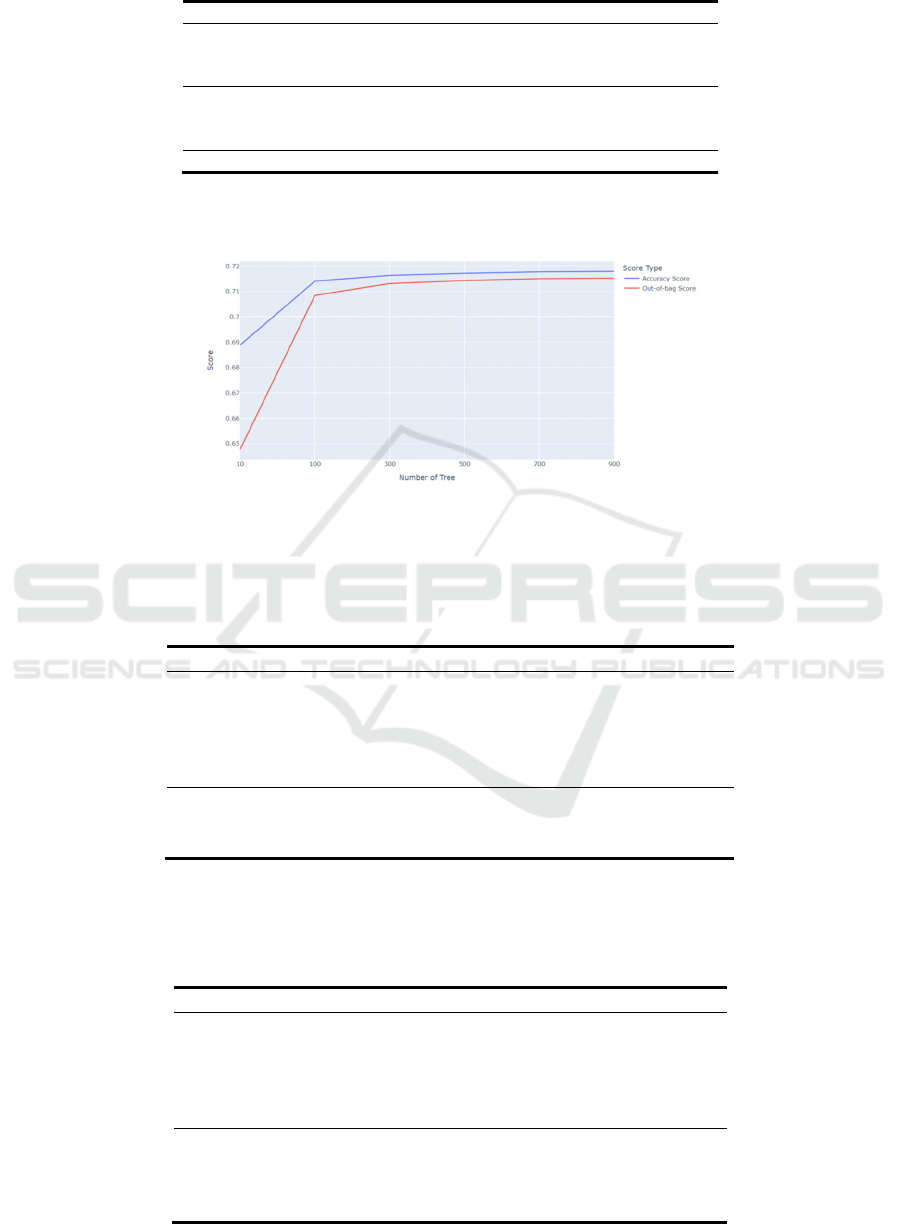
Table 5: RF with default 100 Trees.
p
recision recall f1-score su
pp
ort
1 0.64 0.48 0.55 5025
2 0.72 0.82 0.77 29652
3 0.72 0.60 0.65 17444
accuracy 0.71 52121
macro av
g
0.69 0.63 0.66 52121
weighted avg 0.71 0.71 0.71 52121
CPU times: total: 2min 30s/Wall time: 1min 27s
In this case, the hyperparameter is the number of
trees, therefore the relation of score obtained and the
number of trees is plotted:
Figure 10: Score for 10, 100, 300, 500, 700, 900 Trees.
As can be seen in Figure 10, the performance
tends to be steady after 100, thus sticking to the
default 100 trees setting. Now the same pattern is
applied to V2:
Table 6: DT with default parameters.
precision recall f1-score support
1 0.44 0.46 0.45 15763
2 0.22 0.23 0.22 17451
3 0.26 0.27 0.26 27283
4 0.33 0.33 0.33 36769
5 0.53 0.51 0.52 55153
accuracy 0.38 152419
macro avg 0.36 0.36 0.36 152419
weighted avg 0.39 0.38 0.39 152419
Though better than random guessing, obviously
0.38 is a poor precision. This is largely due to the
removal of post-eq features. The result incorporating
these features is instead pretty good:
Table 7: The result incorporating the features.
precision recall f1-score support
1 0.90 0.90 0.90 15763
2 0.71 0.72 0.71 17451
3 0.65 0.65 0.65 27283
4 0.77 0.76 0.76 36769
5 0.96 0.96 0.96 55153
accuracy 0.82 152419
macro avg 0.80 0.80 0.80 152419
weighted
avg
0.82 0.82 0.82 152419
PMBDA 2022 - International Conference on Public Management and Big Data Analysis
140

However, as explained before, these features
should not be included. Therefore, V2 will no longer
be considered in the prediction. Results based on V1
will be compared and discussed instead.
RF beats the default DT in accuracy; Results are
close when DT is finely tuned (That means most
subtrees give the same result as DT, so aggregating
votes is no more an advantage); DT runs much faster
than RF.
As the reports suggest, the recall rate of grade 2 is
the highest, followed by grade 3 and grade 1, which
generally matches the damage grade distribution of
V1 in Figure 1, in other words, the amount of training
for each damage grade. This is one of the effects of
skewed data. The data skew primarily refers to a non-
uniform distribution in a dataset (Bouganim, Data
Skew, Liu, Özsu 2017).
4 CONCLUSION
Based on 2 versions of the same earthquake data, this
paper studies the connection between building
characteristics and earthquake damage through data
analysis and machine learning. Key points are
summarized in two parts. From the EDA part, first,
age is positively correlated with the damage grade,
but it is not a strong indicator alone; second, smaller
buildings generally tend to have a higher damage
grade which should be given more focus in disaster
relief; third, more attachments lead to less destruction
generally; fourth, improving material quality should
be a top priority in the area and traditional manners
should be considered during the construction. By
doing so, the risk of being highly destructed can be
lowered to 1/8 under a similar situation. From the ML
part, the training data from V1 and DT with optimal
parameters are used for better results and less time
consumption of the prediction.
In this paper, the overall prediction accuracy rate
is 0.72. Actually, the precision of grade 3 is the most
important in targeted disaster relief. As shown in the
reports above, the recall of grade 3 is around 0.6. To
improve it further, it is better for future work to find
a dataset with a bigger proportion of a high damage
grade, a bigger data volume, and possibly a better
choice of features.
REFERENCES
Arya, A. S.: Guidelines for Earthquake Resistant Non-
Engineered Construction, International Association for
Earthquake Engineering (1994).
Busuttil, S.: Support Vector Machines, 34-39 (2003).
http://www.cs.um.edu.mt/~csaw/CSAW03/Proceeding
s/SupportVectorMachines.pdf.
Berrar, D. Bayes’ Theorem and Naive Bayes Classifier
(2018). 10.1016/B978-0-12-809633-8.20473-1.
Breiman, L. Random Forests. Machine Learning 45, 5-32
(2001). https://doi.org/10.1023/A:1010933404324.
Bouganim L.: Data Skew. L. Liu; M.T. Özsu. Encyclopedia
of Database Systems (2nd edition), Springer, 634-635
(2017). 978-0-387-35544-3. ff10.1007/978-1-4899-
7993-3_1088-2ff. ffhal01656691v2f.
Refaeilzadeh, P., Tang, L., Liu, H.: Cross-Validation. In:
LIU, L., ÖZSU, M.T. (eds) Encyclopedia of Database
Systems. Springer, Boston, MA (2009).
https://doi.org/10.1007/978-0-387-39940-9_565.
Ranjan, G. S. K., Verma, A. and Sudha, R.: K-Nearest
Neighbors and Grid Search CV Based Real Time Fault
Monitoring System for Industries. 1-5 (2019).
10.1109/I2CT45611.2019.9033691.
Song, Y. Y., Lu, Y.: Decision tree methods: applications
for classification and prediction. Shanghai Arch
Psychiatry 27(2), 130-5 (2015). doi:
10.11919/j.issn.1002-0829.215044.
White, H.: A Reality Check for Data Snooping.
Econometrica 68, 1097-1126 (2000).
https://doi.org/10.1111/1468-0262.00152.
Wang, C. K., Salmon, C. G.: Reinforced Concrete Design,
National Academics (1979).
https://trid.trb.org/view/502701.
Analysis of the Seismic Destructive Force and Building Features with Tree-Based Machine Learning
141
